blog

Events: A thing that can happen

Experiments: Have events as outcomes

• If outcomes can come from set A or B, then the total number of outcomes is:

• If outcomes are generated via a process with r steps, where step i has ni outcomes, then the total number of outcomes is: n1 * n2 * … * nr

• sort objects (permutation)
  • distinct: if n is the total number of elements to sort, then the total number of ways to sort is n!
  • semi-distinct: if there are n objects, n1 are the same (within the group), n2 are the same (with in the group) … then there are unique orderings (permutations)
• choose k objects (combinations) from distinct items
  • for instance, there are n = 20 people, choose k = 5 people to get cake and the ordering of those 5 does not matter
  • 
• put objects into r buckets
  • items are distinct: r^n where n is number of items
  • items are not distinct:

• 0 <= P(E) <= 1
• P(S) = 1
• P(E^c) = 1 - P(E) or P(E union F) = p(E) + p(F) if event E and F are mutually exclusive

• written as P(E|F) : means P(E, given F already observed)
• the definition of conditional probability: , this holds even when outcomes are not equally likely
• In general:
• 
• machine learning is: probability + data + computers

• 
• Bi are mutually exclusive

• 
• it is also equal to the above equation after applying low of total probability
• update belief
  • we have some P(location) before observation, know P(observation|location), update P(location)
  • after observation, we want to compute P(L|O), use bayes theorem and law of total probability to compute it

• if two events E and F are mutually exclusive, then P(E union F) = P(E) + P(F)
• if two events E and F are not mutually exclusive, then P(E union F) = P(E) + P(F) - P(EF)
• for three sets, P(E union F union G) = P(E) + P(F) + P(G) - p(EF) - p(EG) - P(FG) + P(EFG). So if there is no mutually exclusion, life will be hard
• two events A and B are independent if P(AB) = P(A)P(B) otherwise they are dependent events. Another definition for indepedent is P(A|B) = P(A)
• if events A and B are independent, prove that A and B compliment are independent
  • the first equality comes from lawy of total probability, P(A) = P(ABc) + P(AB)
• general definition of independence is that for verey subset with r elements, P(E1…Er) = P(E1)…P(Er)
• example, p is the probability to get head by rolling a dice, what is P(exactly k heads on n coin flips)
  • each coin flip are independent and the probablity of getting one case of k head is:
  • so the total probablity is:

• DeMorgan’s laws: ;

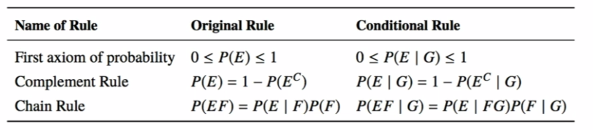
• in the conditional paradigm, the formulas of probability are preserved
• , similar to the previous equation, just add condition on E for every term
• independence relationships can change with conditioning (if events E and F are independent, that does not mean they will still be independent given another event G)
• two events E and F are conditionally independent given G if P(EF|G) = P(E|G)P(F|G) or P(E|FG) = P(E|G)

• for instance, Y = number of “heads” on 3 coins. Y is a random variable, Y could be 0, 1, 2, 3
• with random variable, we can do:
  • probability mass function P(X=a) which means the probability of a random variable take particular value. Can think of it as a function, given a value, output a probability. Notice the random variable is discrete
    • the notation could also be written as p(x) or
  • expectation E[X]
    • for discrete random variable X: , in other words, sum over all values of x that have PMF bigger than 0
    • other semantic meaning: mean, weighted average, center of mass, 1st moment
    • properties:
      • linearity: E[aX+b] = aE[x] + b
      • expectation of a sum is the sum of expectations: E[X + Y] = E[X] = E[Y]
      • unconscious statistician:
  • variance: Var(X)
    • think about value x and the difference to the mean E[x]. How to get the average difference, one way is to do average of the absolute value of difference (L1 norm); the other way is to average over the square of the difference (L2 norm)
    • we use L2 norm in variance and variance is a formal representation of “spread”
    • for X being a random variable = =
    • standard deviation is the square root of variance
    • also called 2nd central moment
    • properties of variance:
      • var(aX+b) = a^2Var(x)
• Bernoulli Random Variable
  • experiment results in either “success” or “failure”
  • P(X=1) = p, P(X=0) = 1-p; X is a Bernoulli Random variable denoted as X ~ Ber(p)
  • E[X] = p, Var(X) = p(1-p)
  • some examples in the real world: coin flip, random binary digit
• Binomial Random Variable
  • consider n independent trials of Ber(p) random variable, X is number of successes in n trials
  • In this case, X is a Binomial Random Variable: X~Bin(n,p)
  • P(X=i) = p(i) = , i=0,1…n
  • the summation of P(X=i) for all i is 1
  • some examples in the real world: # of heads in n coin flips, # of 1s in randomly generated length n bit string
  • E[X] = np, Var(X) = np(1-p)
  • Ber(p) = Bin(1,p)
  • Galton Board, if we want to represent whether a particular marble goes right, it is a Bernoulli random variable R~Ber(0.5); if we look at what bucket a marble lands in, then it is binominal random variable B~Bin(levels, 0.5)

• A formulat that is about natural experssion:
• one usage of it is to determine the probability of haveing n requests if given lambda = k requests among a region in one minute
  • we can model this as a binominal distribution. If the granularity is second, then it can be expressed as X~Bin(60, k/60)
  • if the granularity is milisecond, it can be expressed as X~Bin(60000, k/60000)
  • if the granularity is so small, we have X~Bin(infinity, k/infinity)
• Binomial in the limit:
  • 
  • equation 2 to 3 uses natural expression
  • equation 4 to 5 uses limit analysis, since n is large n!/(n-k)! = n^k
• Poisson Random variable: the number of occurrences in a fixed interval of time
  • X ~ Poi(lambda)
  • lambda is the “rate”
  • X takes on values 0,1,2..
  • it has PMF P(X=k) =
  • usage: earthquakes, radioactive decay, hits to web server; have time interval for events
  • discrete
  • events are independent
  • Poisson is greate when you have a “rate” and make sure the rate has the correct unit that is asking
  • Poisson can be used to approximate Binominal when n is large, p is small. lambda = n*p (we expect np to be moderate large, such as n>20, p<0.05)
  • X ~ Poi(lambda) where lambda = np (n->infinity, p -> 0)
    • E[X] = np = lambda (recall the expectation of binomial distribution)
    • Var(x) = np(1-p) = lambda * (1-0) = lambda
  • Can still apply Poisson approximation when independent assumption (or same probability p) is “mildly” violated
    • number of entries in each bucket in large hash table
    • average number of requests to web server
    • Notice that the PMF can be adapted if, instead of the average number of events \lambda , we are given a time rate r for the events to happen. Then lambda =rt with r in units of 1/time, and

A midpoint summary

|                  | number of successes | number of time to get success |
|------------------|---------------------|-------------------------------|
| one trial        | X~Ber(p)            | X~Geo(p)                      |
| several trials   | X~Bin(n,p)          | X~NegBin(r,p)                 |
| interval of time | X~Poi(lambda)       | X~Zipf                        |

• X is number of independent trials until first success
• p is probability of success on each trial
• 
• E[X] = 1/p
• Var(X) = (1-p)/p^2

• X ~ NegBin(r,p)
• X is number of independent trials until r successes
• p is probability of success on each trial
• P(X=n) = where n = r, r+1…
• E[X] = r/p
• Var(X) = r(1-p)/p^2
• Geo(p) ~ NegBin(1,p)

• You “mine a bitcoin” if for given data D, you find a number N such that Hash(D, N) produces a string that starts with g zeros. Solve using geometric random variable equation.

• The probability density function (PDF) of a continous random variable represents the relative likelihood of various values. or in a different notation
• Properties of PDF:
  • the value is >=0, <=1
  • integrate from -infinity to +infinity is 1
  • PDF articulate relative belief, the integration of it is a probability
  • f(X=x) is not a probability, it could be greater than 1
• Expectation:
  • The properties of expectation of discrete RV still hold
• Variance:
• Uniform Random Variable
  • X ~
  • PDF: otherwise f(X=x) is 0
    • 
    • 
• Exponential Random Variable
  • continuous equivalent of Poisson distribution, it represents time we need to wait until some event (such as eqrthquake, request to web server, end cell phone contract etc) given constant rate
  • X ~ , rate \lambda > 0
  • PDF: otherwise f(X=x) = 0
  • E[X] = 1/lambda
  • Var(X) = 1/(lambda)^2
  • support: X>=0
  • for instance if given the rate of earthquick per year, ask what is the probability of having zero major earthquake next year, use poisson; if ask what is the probability of a marjor earthquake in the next 30 years, use exponential RV
• Cumulative Density Function: it is a “closed form” equation for the probability that a random variable is less than a given value F(x) = P(X<x). It can be used to avoid integrals
  • Short hand notation:
  • the CDF of exponential RV is:
• A quick notation summary:
  • p(a) or p_{X}(a): probability mass function (discrete) P(X=a)
  • f(a) or f_{X}(a): probability density function (continuous) f(X=a)
  • F(a) or F_{X}(a): cumulative distribution function P(X<=a)
• Normal distribution
  • X ~
  • PDF: f(x) = where -\infinity < x < \inifinity
  • E[X] = \mu
  • Var(X) = \signma ^2
  • Also called Gaussian, f(x) is symmetric about \mu
  • why use normal distribution:
    • common for natural phenomena (such as heights, weights) (it is log-normal in reality)
    • often results from the equally weighted sum of multiple variables
    • most noise is normal (at least assumed to be normal)
    • means of samples are distributed normally
    • more importantly, it is the least assuming distribution (simple and will generalize). It maximizes entropy (measures mathematical disorder) for a given mean and variance
  • No colosed form for CDF
  • Look up table method: F(x) = where \phi is a function that has been solved for numerically for \mu = 0, \sigma = 1 (standard normal)
  • Linear Transformation of normal is normal. Y = aX + b is also normal if X is normal. E[Y] = aE[X] + b; Var[Y] = a^2 \sigma ^2. So Y ~ N(a \mu + b, a^2 \sigma ^ 2)
    • a special case of linear transform: Z = (X - \mu)/(\sigma) ~ N(0,1). This is called the standard normal distribution.
      • \phi (-a) = 1 - \phi(a)
      • P(c < Z < d) = \phi (d) - \phi (c)
  • So for X ~ N(\mu, \sigma ^2), it is equal to \phi((x-\mu)/ \sigma)

• relative probability: ratio of probability. For instance P(X=10)/P(X=5) = deltaf(X=10)/deltaf(X=5) = f(X=10)/f(X=5) and use the PDF formula to get the ratio. The delta technique is used here to simulate integration
• Normal approximations binomial. For instance Bin(100, 0.5) ~ Normal(50,25) since E[X] = np, Var(X) = np(1-p)
  • one nuance about the approximation is about continuity correction. Discrete think about decimals but continous are not. Think about how it is around and where to start to integrate. For instance to get P(X>=65), we might need to integrate from 64.5 if using continuous approximation.

  • A table of continuity correction:

    | Discrete probability question | Continuous probability question |
    |-------------------------------|---------------------------------|
    |              X=6              |            5.5<Y<6.5            |
    |              X>=6             |              Y>5.5              |
    |              X>6              |              y>6.5              |
    |              X<6              |              Y<5.5              |
    |              X<=6             |              Y<6.5              |
    

  • can approximate binomial when n large (>20), p is mid-ranged (np(1-p)>10)
  • recall poisson can also approximate binomial when n large (>20), p small (<0.05)
  • general idea: if there is a choice, go with the normal approximation

• RV interact with each other
• notation P(A=1, B=1): probability that A takes value 1 and B takes value 1
• For two discrete random variables X and Y, the joint probability mass function is:
• Marginal distributions: ;
• Multinomial distribution
  • n independent trials of experiment performed
  • each trial results in one of m outcomes with probabilit p1…pm
  • Xi = number of trials with outcome i
  • . LHS is a joint distribution, the first term in RHS represents multinomial number of ways of ordering the successes; the second term in RHS means probabilities of each ordering are equal and mutually exclusive. c1 + … + cm = n and
  • binomial: each trail has 2 possible outcomes; multinomial: each trial has m possible outcomes. It is a generalization of binomial
  • one interesting view in probabilistic text analysis: there are about 988,969 words in english. Can think of text as rolling a die with that amount of outcomes. So in this point of view, text is a multinomial.

• A joint probability density function gives the relative likelihood of more than one continuous random variable each taking on a specific value
• Marginal probabilities give the distribution of a subset of the variables (often just one) of a joint distribution
• notation summary:
  • joint probability: or P(X=a, Y=b)
  • continuous joint probability density: or f(X=a, Y=b)
  • single (marginal) probability density function: or f(X=a)
  • single probability mass function: or P(X=a)

• Say we know the articles written by A and B, we want to determine who writes article of C
• from articles of A, we can get hi = probability that A writes word i (just count the number of times word i appears and divide the total number of words)
• from articles of B, we can get mi = probability that B writes word i

• we compare P(A

  C) and P(B

  C) which every is larger, then C is written by whom

• , P(A) is our prior belief. Since we don’t have prior knowledge about A and B, we set P(A) = P(B) = 1/2
  • P(C|A) can be think of as a multinomial distribution, A is like a bag of words, C is a distrubtion of some of its words. So P(C|A) = where ni is the number of times wordi appears in document C

  • P(C) is hard to manipulate but if we take the ratio of P(A

    C) and P(B

    C), it will be canceld

• 
• to avoid the number being too small, we can take the log and do:
• the method here is similar to text classification in naive bayes

• jointly continuous function:
• cumulative density function in jointly continuous RV (jointly CDF):
• using joint CDF, we can avoid integral while computing the joint PDF:
• discrete conditional distributions
  • if X and Y are discrete random variables, conditional PMF of X given Y is:
• continuous conditional distributions
  • let X and Y be continuous random variables, use PDF to compute conditional joint probability. The idea is that we can turn PDF to probability by multiply a small distance epsilon and it will cancel out. So
• Bayes revisited:
  • P(B|E) is called posterior belief; P(E|B) is the likelihood of evidence; P(B) is prior belief; P(E) is normalization constant.
• Mixing discrete and continuous:
  • Let X be a continuous random variable, let N be a discrete random variable, consider
  • We have
  • Again the idea is the same, for continuous RV, we use PDF times epsilon; for discrete RV, we use PMF directly
  • Similarly, the LHS can also be PMF and RHS has PDF. Or it can all be continuous, all have PDF
• Bivariate normal:
  • X,Y follow a symmetric bivariate normal distribution if they have joint PDF:
    • 
    • it is a 2D Gaussian
• continuous conditional joint probability
  • goal f(X=x, Y=y | D=d)
  • X and Y are Gaussian, we have f(X=x, Y=y) which is prior
  • we have f(D=d | X=x, Y=y), D is observation
  • where f(D=d) is just a constant for a given d because it is not based on x and y
• expectation of multiple RVs
  • expectation over a joint isn’t nicely defined because it is not clear how to compose the multiple variables
  • lemma: for a function g(X,Y) we can calculate the expectation of that function:
    • E[g(X,Y)] =
    • recall for a single RV: E[g(X)] =
• independence of RVs
  • two discrete random variables X and Y are independent if: P(X=x, Y=y) = P(X=x)P(Y=y)
  • to check independent of RVs, the above equation need to hold for all combinations of RVs
    • but for an event, it just need to hold for one combination
  • intuitively: knowing the value of X tells us nothing about the distribution of Y (and vice versa)
  • for continuous variables
    • two continuous RVs X and Y are independent if:
      • P(X<=a, Y<=b) = P(X<=a)P(Y<=b) for any a,b
      • or for any a,b
      • or factorize CDF:
      • more generally joint density factors separately where x>-\infinity y<\infinity
• Insight to convolution which is the interaction (such as addition, subtraction) of RVs
  • Let X be the amount of points you score, let Y be the amount of points your opponent socres
    • Say you know P(X=x) and P(Y=y)
    • what is the probability of a tie?
      • P(tie) =
  • what about X+Y=n?
    • similar idea: P(X+Y=n) =
    • in continuous case: f(X+Y=alpha) =

• the intent is to solve how each RV is related to each other
• sum of independent RVs
  • for X ~ Bin(n1, p), Y ~ Bin(n2, p)
    • X + Y ~ Bin(n1+n2, p)
  • for X ~ Poi(lambda1), Y ~ Poi(lambda2)
    • X + Y ~ Poi(lambda1 + lambda2)
  • for normal distribution X ~ N(u1, sigma1^2), Y ~ N(u2, sigma2^2)
    • X + Y ~ N(u1+u2, sigma1^2 + sigma2^2) notice this hold only if X and Y are independent
    • X is dependent on X, so 2X is not N(2u1, 2sigma1^2), instead it is N(2u1, 4sigma1^2)
• vary together
  • (x-E[x])(y-E[y]) positive means x and y vary together
• Covariance of X and Y
  • we are not only look at (x-E[x])(y-E[y]) but the expectation of it since (x-E[x])(y-E[y]) could cancel itself in a distribution
  • Cov(X,Y) = E[(X-E[X])(Y-E[Y])]
  • covariance is used to quantify how two RVs vary together
  • simplify Cov(X,Y) = E[XY - E[X]Y - XE[Y] + E[Y]E[X]] = E[XY] - E[X]E[Y] - E[X]E[Y] + E[X]E[Y] = E[XY] - E[X]E[Y]
  • if X and Y are independent, E[XY] = E[X]E[Y], so Cov(X,Y) = 0
  • but Cov(X,Y) = 0 does not mean X and Y are independent
  • properties
    • Cov(X,Y) = Cov(Y,X)
    • Cov(X,X) = E[X^2] - E[X]E[X] = Var(X)
    • Cov(aX+b, Y) = aCov(X,Y)
    • 
• Correlation
  • Cauchy-Schwarz inequality
    • -std(X)std(Y) <= Cov(X,Y) <= std(X)std(Y)
  • say X and Y are arbitrary RVs
    • the correlation of X and Y is defined as:
    • by Cauchy-Schewarz inequalty, rho is in the range of [-1,1]
    • correlation measures linearity between X and Y
    • rho(X,Y) = 1 we can get Y = aX + b where a = sigmay/sigmax
    • rho(X,Y) = -1, we can get Y = ax+b where a = -sigmay/sigmax
    • rho(X,Y) = 0, it means absense of linear relationship, note it does not mean independent. We say it is “uncorrelated”